Quick start

In about ten minutes you will model a simply supported steel beam under a uniform load, read the reactions, shear force and bending moment, and check them against the textbook formulas.

Follow along

Open run.edubeam.app in a second tab. If a model is already there, use Clear mesh in the app bar to start empty, and tick Delete materials and Delete cross sections to start completely fresh. Clearing can be undone with Ctrl+Z, and the old model stays in ☰ → Recent structures.

Prefer to learn by doing with hints on screen? ☰ → Draw your first beam walks you through a similar beam with the mouse.

The problem

A 6 m simply supported beam (pinned at the left, roller at the right) carries a uniform load of 12 kN/m. Material: steel, $E = 210\ \text{GPa}$, $G = 81\ \text{GPa}$. Section: an IPE 200, $A = 28.5\ \text{cm}^2$, $I_y = 1943\ \text{cm}^4$, $h = 200\ \text{mm}$.

1. Check the units

The units chip in the bottom-right corner of the viewer shows the units every input field and result uses. This tutorial assumes the SI defaults: metres, kN, kNm and MPa.

The grid (G), snap (S) and crosshair toggles, and the units chip

If you see ft · kip · kip·ft · ksi, click the chip and choose Unit system → SI (metric).

2. Add the material and cross section

Elements need a material and a cross section, so create those first.

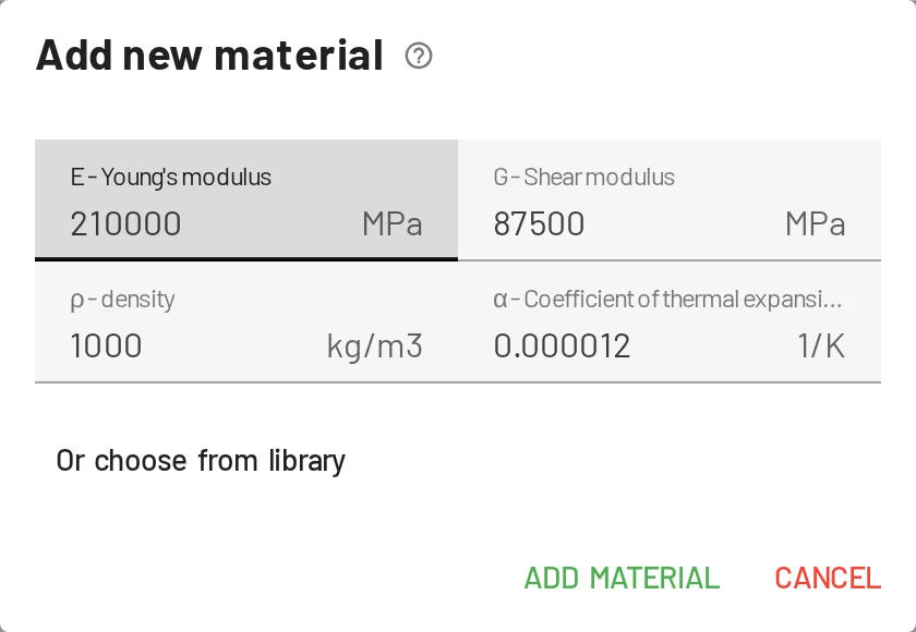
1. Open the Materials tab in the bottom bar and click Add material.
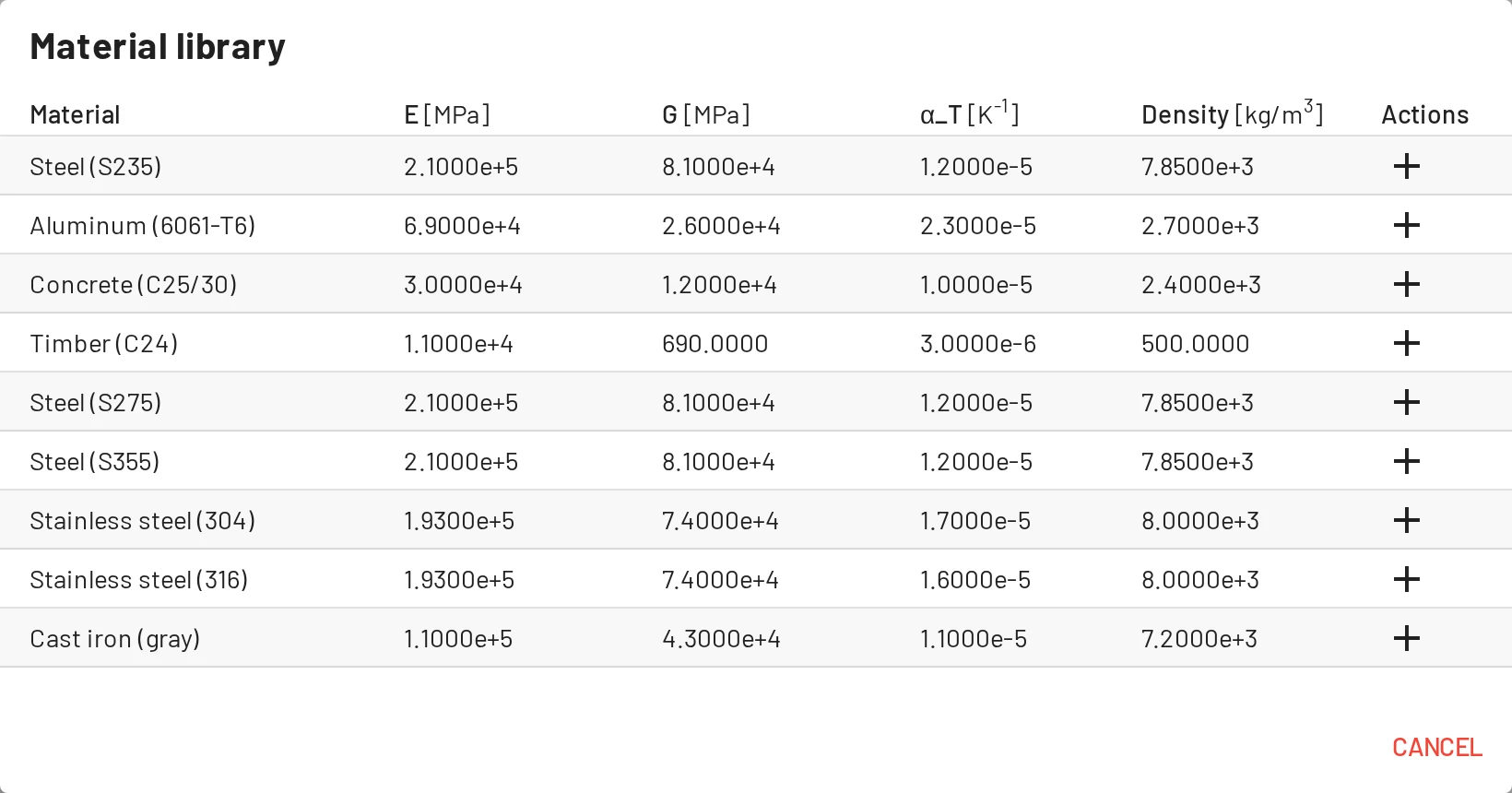
2. Enter E = 210000 MPa and G = 81000 MPa. Leave the density and α = 0.000012 1/K. Click Add material.

Add material: type E and G…

…or pick Steel (S235) from the Material library

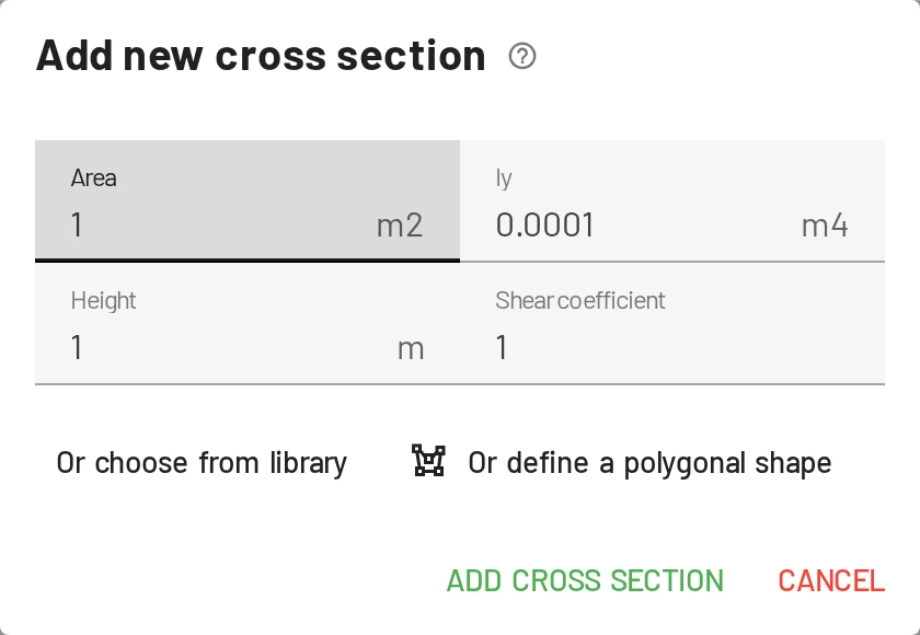
3. Open the Cross sections tab and click Add cross section.
4. Enter Area = 0.00285 m², Iy = 1.943e-5 m⁴, Height = 0.2 m and Shear coefficient = 1. Click Add cross section.

Add cross section. Or choose from the library, or draw a polygonal shape.

Why does the shear coefficient matter?

EduBeam uses Timoshenko beam elements, which include shear deformation. k is the shear correction factor: $k \approx 0.83$ for a rectangle, and about $0.4$–$0.5$ for an I-section when $A$ is the full area. Setting k = 1 with the full area slightly understates shear flexibility. For a slender beam like this one the difference in deflection is well under 1 %. See the beam theory page for the formula.

3. Add the nodes

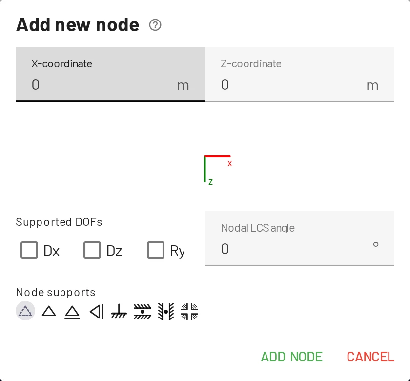
1. Open the Nodes tab. It has two Add node buttons: the first opens a dialog, the second (with a cursor icon) places nodes with the mouse. Click the first.
2. Enter X = 0, Z = 0 and click Add node. The node is labelled 1.
3. Add a second node at X = 6, Z = 0. This is node 2.

The Add node dialog can also set the supports straight away

With the mouse button instead, each click on the canvas places a node. With Snap to grid on (S), clicks land on the grid step (0.1 m by default).

4. Connect them with an element

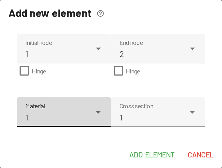
1. Open the Elements tab and click the first Add element button.
2. Choose Initial node 1 and End node 2. Your material and cross section are already selected. Click Add element.

Add element: the two end nodes, optional end hinges, material and section

A line appears between the nodes. Press F to fit it to the screen.

5. Add the supports

In the Nodes tab, the Supported DOFs column has a support-symbol picker and three checkboxes per node: Dx, Dz, Ry.

• Node 1: pick the pin symbol, or tick Dx and Dz.
• Node 2: pick the roller, or tick Dz only.

Supports in the Nodes table: node 1 pinned, node 2 on a roller

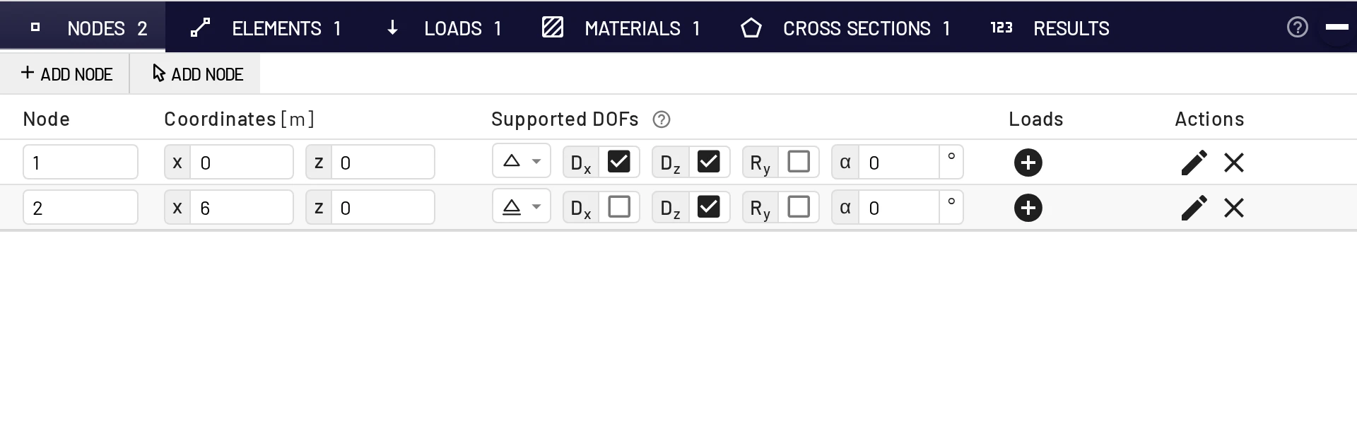
You can also click a node in the viewer and choose Node supports. Nodes & supports lists every support type.

6. Add the load

1. Open the Loads tab and click Add element load.
2. Load type: Uniformly distributed load. Element: 1.
3. Enter fz = 12 kN/m and leave fx = 0. Click Add element load.

The dialog previews the load on the element

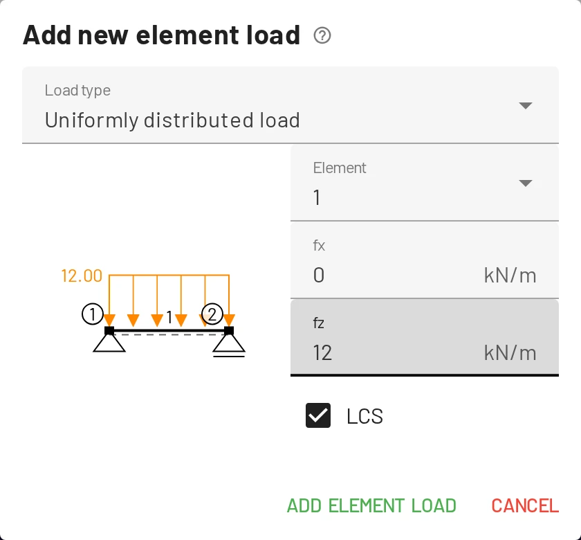
Positive fz points in the +z direction, which is down on screen, so a positive value is a gravity load. See the sign conventions.

7. Read the results

The solution appears as soon as the load is added. The display panel at the top right of the viewer switches the diagrams on and off. Deformed shape, M_y(x) and Reactions are on by default. Tick V_z(x) to add the shear force.

Shear force (green), bending moment (red), reactions (purple) and the deformed shape

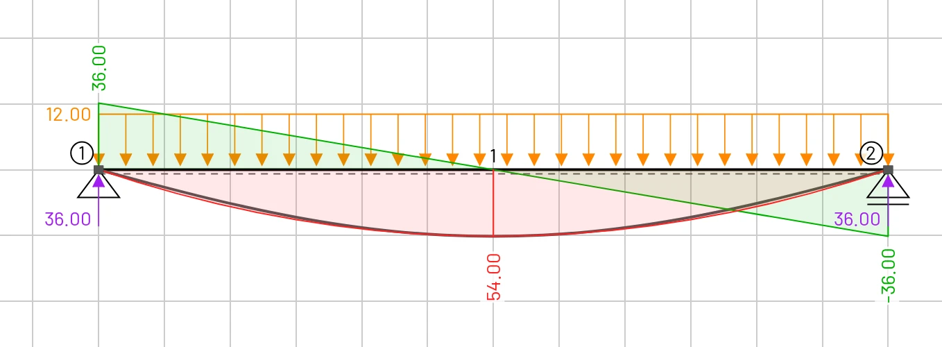
Overlay	What you should see
Reactions	Two upward arrows of 36 kN at nodes 1 and 2.
Vz(x)	A straight line from +36 kN at the left to −36 kN at the right, crossing zero at mid-span.
My(x)	A parabola with its extreme of 54 kNm at mid-span.
Deformed shape	A symmetric sag. Point at node 1 to read its rotation: 2.6469 · 10⁻² rad.

The Results tab in the bottom bar gives the numbers. Nodal results lists Dx, Dz, Ry for each node. Element results lists the end forces of each element in its local coordinate system.

If the diagrams look too large or too small, change Results scale in Settings → Viewer settings → Sizes.

8. Check by hand

Quantity	Formula	Hand value	EduBeam
Reaction	$R = qL/2$	36 kN	36 kN
Max shear	$V = qL/2$	36 kN	36 kN
Max moment	$M = qL^2/8$	54 kNm	54 kNm
End rotation	$\varphi = qL^3/(24EI)$	0.02647 rad	0.02647 rad
Mid-span deflection (bending)	$w = 5qL^4/(384EI)$	49.63 mm
Mid-span deflection (shear)	$w_s = qL^2/(8kGA)$	0.23 mm
Mid-span deflection (total)	sum	49.86 mm	49.86 mm

There is no node at mid-span, so to read the deflection there, add one: choose the second Add node button, click on the beam at X = 3 and pick Connect to structure. The beam is split in two and the new node's Dz in Results reads 49.86 mm. Splitting does not change any result, because the element is exact.

Everything matches. More hand-check recipes (cantilever, fixed beam, truss, temperature) are in Checking results by hand.

9. Experiment

This is where EduBeam earns its keep. Try each of these and watch the diagrams update:

• Drag node 2 to the right: the moment grows with $L^2$.
• Tick Ry at node 1 to fix it: the mid-span moment drops and a hogging moment appears at the support.
• Tick Dz at the mid-span node you just added, to make a two-span continuous beam.
• Tick an End hinge on an element in the Elements tab to release the moment at one end.
• Press Ctrl+Z to undo any step.

10. Save or share

• Share model (in the app bar or the ☰ menu) gives you a link that contains the whole model. Paste it into an e-mail, a chat or your slides.
• ☰ → Save project (Ctrl+S) downloads a project.json you can open later with Open project or by dropping it onto the app.
• ☰ → Export image (Ctrl+P) saves the drawing as PNG or SVG for a report.

Your model is also kept in the browser, so reloading the page does not lose it. See Import, export & sharing.

Where next

• Three-hinged frame tutorial: a frame with an internal hinge, checked by hand.
• Examples: open ready-made frames and trusses in one click.
• Loads: trapezoidal, concentrated and temperature loads, prescribed displacements.
• Keyboard, mouse & touch: work faster on the canvas.