Functions
Everything the components draw comes from pure functions with no Vue in them. They write a figure as an SVG file, read results exactly, prepare data ahead of time, and build figures of your own. Named imports keep a bundle small: a page that imports only modelFromSolver gets no component code at all.
All values are SI unless a unit says otherwise; positions along a member are metres from its start node.
A standalone SVG file
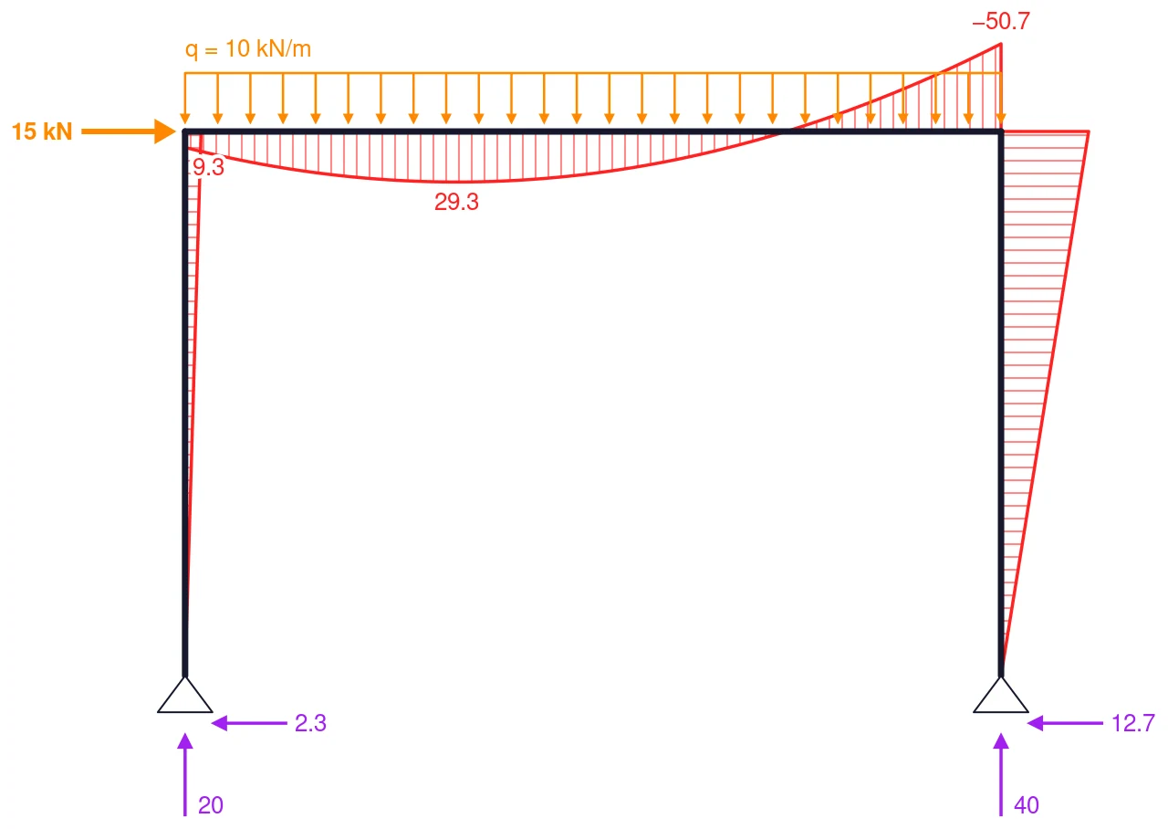
A plot in a page takes its colours from the page's CSS custom properties, so an <svg> copied out of it has none. structureSvg writes the figure as the text of a standalone .svg file instead: plain colours, no stylesheet, no scripts, laid out by the same routine as StructurePlot. Word, PowerPoint, Inkscape, CairoSVG and LaTeX tool chains draw it as the page does.
import { writeFileSync } from 'node:fs'
import { modelFromSolver, structureSvg } from '@edubeam/plot'
import { portalFrame } from './frame.ts' // () => a solved LinearStaticSolver, as on the Slides page

const frame = modelFromSolver(portalFrame())
writeFileSync('frame.svg', structureSvg(frame, { layers: ['members', 'supports', 'loads', 'reactions', 'M'] }))
| Option | Default | What it does |
|---|---|---|
layers | members, supports, loads, reactions and the result StructurePlot would pick | What to draw |
width | 640 | Width in px, the SVG's user units |
height | follows the drawing | A fixed height, px |
maxHeight | max(320, 0.75 × width) | The upper bound of the automatic height |
padding | 6 | Space around the drawing, px |
fontSize | 13, compact 11.5 | Text size, px |
fontFamily | Helvetica, Arial, sans-serif | A font stack the program opening the file has |
colors | PRINT_COLORS | Any of the tones, as plain colours |
background | true | Paint the background in paper; false leaves it transparent |
title | none | Written as the SVG's <title> |
reserve, reserveLabelModes, reserveReactionLabels | none | Layers, label styles and reaction label styles to make room for besides those drawn, so the files of a build-up line up: A build-up in Beamer |
units, numberFormat, compact, diagramSize, deformedSize, momentOnTensionSide, resultLabelMode, reactionLabels | as StructurePlot | The same meaning as the component's props |
PRINT_COLORS are the EduBeam app's colours on white: ink #16182b, normal force #2222ff, shear force #00af00, bending moment #ff2222, loads #ff8700, reactions #a020f0. Every label is written twice, a halo in the background colour under the text, because not every SVG program understands paint-order, and a subscript, as in the reaction names Ax, is a tspan with plain numbers that Word and Inkscape read. Without reserve, a file is fitted to the layers it draws.
To use the file:
- Word and PowerPoint (2019 and Microsoft 365): Insert › Pictures.
- LaTeX: convert it to PDF with CairoSVG (
cairosvg frame.svg -o frame.pdf) or Inkscape, then\includegraphics; or use\includesvgfrom thesvgpackage, which calls Inkscape for you. At 640 units wide, a figure set to a 16 cm text column has 9 pt labels. - A web page without Vue: paste the text into the HTML. See Without Vue.
Exercises and tests writes a file for every student's exercise and key.
From a solver
| Export | Signature | Does |
|---|---|---|
modelFromSolver | (solver: Solver, options?: FromSolverOptions) => PlotModel | Reads a solver into the plain plot model; results only for a solved load case |
FromSolverOptions | type | { loadCase?: number }, an index into solver.loadCases |
Piecewise polynomials
A member's results are Piecewise values: lists of { x0, x1, c } pieces, explained in Plot model. side picks the value just before ('left') or just after ('right', the default) a point where two pieces meet.
| Export | Signature | Does |
|---|---|---|
valueAt | (pw, x, side?) => number | The value at x; past the ends, the nearest end value |
slopeAt | (pw, x, side?) => number | The derivative, value units per metre |
extremes | (pw) => { max: Extreme; min: Extreme } | null | The largest and smallest value, exactly, each { x, value, side } |
maxAbs | (pw) => number | The largest absolute value |
innerBreaks | (pw) => number[] | Where pieces meet, without the two ends |
isZero | (pw) => boolean | Whether the result is zero throughout |
evalPiece | (piece, x) => number | The value of one piece |
evalPieceSlope | (piece, x) => number | The slope of one piece |
pieceExtrema | (piece) => number[] | Where the slope of a piece is zero, m |
pieceDegree | (piece) => number | null | The degree of a piece; null when it is zero |
cleanPiecewise | (pw, tolerance) => Piecewise | Drops coefficients below tolerance, the round-off of a solved model |
fitPiece | (f, x0, x1, degree) => Piece | The polynomial of a degree through a function on (x0, x1) |
pieceToBeziers | (piece, segments?) => CubicSegment[] | The piece as cubic Béziers in (x, value): exact up to cubics, else segments of them, 4 by default |
Types: Piece, Piecewise, Side ('left' \| 'right'), Extreme, CubicSegment.
Units and numbers
| Export | Signature | Does |
|---|---|---|
KN_UNITS | Units | kN, kNm, kN/m, m, mm, mrad, K: the default |
SI_UNITS | Units | N, N·m, N/m, m, m, rad, K |
resolveUnits | (units?: Partial<Units>) => Units | KN_UNITS with your overrides |
DEFAULT_NUMBER_FORMAT | Intl.NumberFormat | English, at most one decimal |
formatNumber | (value, format?) => string | The number with a true minus sign, never −0 |
formatQuantity | (si, unit, format?) => string | "36 kN": an SI value in a unit, with a narrow no-break space |
A Unit is { symbol, scale }, display value = SI value × scale. Units has one for each UnitKind: force, moment, distributed, length, displacement, rotation and temperature.
import { formatQuantity, KN_UNITS } from '@edubeam/plot'

formatQuantity(-37500, KN_UNITS.moment) // "−37.5 kNm"
Reading values
| Export | Signature | Does |
|---|---|---|
readMember | (results: MemberResults, x, snap?) => { x, u, values } | N, V, M and w at x, each { left, right }, and the axial displacement u; snaps to a step within snap m |
readoutAt | (model, transform, px, py, reach) => Readout | null | The member nearest a screen point within reach px, and its results there |
readoutMarks | (model, transform, readout, shown, k, side) => ReadoutMark[] | Where the read values are drawn: each shown diagram's ordinate tip (both across a step), the point on the deformed shape |
formatReadout | (readout, quantity, units, format?) => string | "M = 54 kNm", or "V = 13.3 → −6.7 kN" across a step |
k is px per SI unit for each result and side the side each diagram is drawn on, from diagramScales and diagramSide below. Types: Readout, ReadoutMark ({ tone, from, to } in px), ReadoutQuantity ('N' \| 'V' \| 'M' \| 'w'), SidedValue.
Beam lines
The pieces of DiagramStack, for building a stacked figure of your own.
| Export | Signature | Does |
|---|---|---|
beamLine | (model, ids?) => BeamLine | The members as one horizontal line, left to right; throws for anything else |
lineDiagram | (model, line, row) => Piecewise | One result along the whole line, in the line's x |
rowRange | (pw) => [number, number] | The range a row is scaled to, always including zero |
rowPeaks | (pw) => RowPeak[] | The extremes worth writing on a row |
rowBreaks | (pw) => number[] | Where the result breaks: supports, joints and point loads |
rowOutline | (pw, sx, sy, close) => string | SVG path data of a row's outline, given the maps from m and value to px |
rowOrdinates | (pw, sx, sy, spacing) => string | SVG path data of the hatching ordinates, spacing px apart |
lineModel | (model, line, omit?) => PlotModel | The model cut down to the line, optionally without one load |
pointLoadAt | (model, line, at) => PlotLoad | undefined | The point force at line position at |
Types: BeamLine, LineMember, RowPeak, StackRow.
The DiagramStack page uses beamLine, lineDiagram and rowRange to keep each row's scale over every position of a moving load.
Geometry and supports
| Export | Signature | Does |
|---|---|---|
nodeMap | (model) => ReadonlyMap<string, PlotNode> | Nodes by id |
memberFrame | (model, member, nodes?) => MemberFrame | A member's start, unit tangent, unit local z and length |
memberFrames | (model) => Map<string, MemberFrame> | The same for every member, by id |
pointAlong | (frame, at) => { x, z } | The point at metres along a member |
supportKind | (fixity) => SupportKind | 'fixed', 'pin', 'roller', 'slider', 'rotation' or 'none' |
supportPlacement | (model, node) => SupportPlacement | The symbol for a node and its clockwise turn, degrees |
supportGlyph | (kind) => readonly GlyphPart[] | The symbol's lines, in px |
glyphReach | (kind, rotation, x, z) => number | How far a turned symbol reaches along a direction, px |
Drawing
The drawing works in three steps. buildStructureScene turns a model into scene items: model points with offsets in screen pixels. fitScene finds the scale and offset that fit them in a box. resolveScene turns them into SVG path data, circles, and the labels that have room. layoutStructure runs all three as StructurePlot and structureSvg do, so a figure of your own is laid out like theirs.
| Export | Signature | Does |
|---|---|---|
layoutStructure | (model, options, box, shown?, labelModes?) => StructureLayout | The whole layout: fit with every label, drop crowded labels, fit again. Returns { fit, items, resolved } |
structureSvg | (model, options?) => string | A standalone .svg file: above |
buildStructureScene | (model, options: StructureSceneOptions) => SceneItem[] | The drawing of the chosen layers at a scale, px per metre |
fitScene | (items, box: FitBox) => Fit | Scale and offset to fit a box { width, height?, maxHeight?, padding, fontSize } |
resolveScene | (items, transform, options: ResolveOptions) => ResolvedScene | { paths, circles, texts } in px, with the labels that fit |
placeLabels | (items, transform, options: ResolveOptions) => Map<SceneText, SceneText> | Which labels to keep, and where |
alternativeResultGroups | (shown) => ReadonlySet<string> | The result layers that are shown one at a time, whose labels give way to the rest but not to each other |
sceneBounds | (items, scale, fontSize) => Bounds | The extent of a scene, px |
project | (transform, anchor) => [number, number] | A scene point on screen, px |
defaultResultLayer | (model) => ResultLayer | null | The result a plot shows when none is asked for |
diagramScales | (model, options) => Record<ResultLayer, number> | px per SI unit for each result |
diagramSide | (q, momentOnTensionSide) => 1 | -1 | Which side of a member a positive value is drawn on |
isBarStructure | (model, memberResults) => boolean | Whether N is written as numbers along the bars (a truss) rather than drawn as a diagram |
tipPlacements | (tip, out, mode, gaps?) => TextPlacement[] | The places a value may take beyond an ordinate's tip |
PLOT_LAYERS | readonly PlotLayer[] | Every layer, in paint order |
RESULT_LAYERS | ['N', 'V', 'M', 'w'] | The result layers |
HATCH_SPACING_PX | 7 | The spacing of the diagram ordinates, px |
DEFAULT_COLORS | PlotColors | The default colour of each tone, as CSS: Theming |
PRINT_COLORS | Record<Tone | 'paper', string> | Plain colours for a file, the app's on white |
toneVars | (colors?) => Record<string, string> | The custom properties a plot sets on its root |
PLOT_CSS | string | The CSS rules inlined into each plot |
ResolveOptions are { fontSize, viewport?, exclude?, alternativeGroups?, shields? }: shields are the groups whose lines keep labels off (the diagrams on show), all of them when left out. In layoutStructure, options.layers are the layers to lay out (everything that may be shown, like reserve), shown those on show, and labelModes the label styles to make room for.
Types: StructureSceneOptions, StructureLayout, StructureSvgOptions, SceneItem, SceneText, TextPlacement, ResolvedScene, ResolvedPath, ResolvedText, ResolvedCircle, ResolveOptions, Bounds, Anchor, Transform, Fit, FitBox, Tone, PlotLayer, ResultLayer, ResultLabelMode, ReactionLabels, SupportKind, SupportPlacement, GlyphPart, and the model types of Plot model.